Quick Sort

Operation	Method	Time	Adaptive?	In-Place?	Stable?	Online?
Quick sort	Divide et Impera, Partitioning	$T_{b} (n) = Θ (n l o g (n)), T_{a v g} (n) = O (n l o g (n)), T_{w} (n) = Θ (n^{2})$	N	Y	N	N

Idea

Quick sort belongs to a class of algorithms which use a Divide-et-Impera approach.

Quick Sort

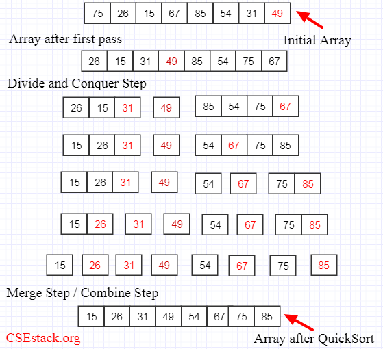
The Algorithm - Divide et Impera

Divide: After choosing a pivot element from $A$ such that $p i v o t (A) = A [q]$ , the vector is partitioned in two sub-vectors $A [p \dots q - 1]$ and $A [q + 1 \dots r]$ (can be empty), such that
1. $\forall A [i] \in A [p \dots q - 1] ∋^{'} A [i] \leq A [q]$
2. $\forall A [j] \in A [q + 1 \dots r] ∋^{'} A [j] \geq A [q]$
3. $A [q]$ is the pivot, the element used to create the partitions and every element that is smaller or larger, is shifted to one of the sub-arrays (so that the conditions are respected).
Impera: sorts the sub-vectors recursively through quicksort, unless the input is trivially small ( $0 \lor 1$ element).
Merge: in this case there is no merge phase, because the algorithm sorts in place

python

quick_sort(Array A, int p, int r)
    if(p < r):
        q = Partition(A, p, r);
        quick_sort(A, p, q-1);
        quick_sort(A, q+1, r);

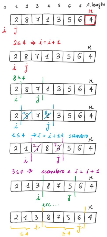
partition(Array A, int p, int r)
    x = A[r];   #Last element
    i = p-1;
    for (j = p to r-1):
        if (A[j] <= x): #Swap if the invariant holds true
            i++;
            swap(A[i], A[j]);
    swap(A[i+1], A[r]); #Put pivot back to the right position
    return i+1;

quick_sort(Array A, int p, int r)
    if(p < r):
        q = Partition(A, p, r);
        quick_sort(A, p, q-1);
        quick_sort(A, q+1, r);

partition(Array A, int p, int r)
    x = A[r];   #Last element
    i = p-1;
    for (j = p to r-1):
        if (A[j] <= x): #Swap if the invariant holds true
            i++;
            swap(A[i], A[j]);
    swap(A[i+1], A[r]); #Put pivot back to the right position
    return i+1;

Invariant

I N V \equiv {\begin{matrix} x = A [r] is always true & \land \\ \forall k \in [p \dots i] ∋^{'} A [k] \leq x & \land \\ \forall k \in [i + 1 \dots j - 1] ∋^{'} A [k] > x & \land \\ p \leq j \leq r & \land \\ p - 1 \leq i \leq j - 1 \end{matrix}

We can confirm this is holds true at all times:

Initialization
Preservation
Conclusion:
- At the end of the for block $j = r$
- This means: $p \leq r \leq r$ and $p - 1 \leq r \leq r - 1$ .
- Furthermore, the last two lines of code in the partition function, insert the pivot in the right position by changing it with the leftmost element larger than x.

I N V [r / j] \equiv {\begin{matrix} x = A [r] is always true & \land \\ \forall k \in [p \dots i] ∋^{'} A [k] \leq x & \land \\ \forall k \in [i + 1 \dots j - 1] ∋^{'} A [k] > x & \land \\ p \leq r \leq r & \land \\ p - 1 \leq i \leq r - 1 \end{matrix}

invariantquicksort

Time Complexity

T_{p a r t i t i o n} (n) = Θ (n) = {\begin{matrix} O (1) & assignments \\ Θ (n) & for block r - p - 1 = n \end{matrix}

And

T_{q u i c k s o r t} (n) = {\begin{matrix} c & n \leq 1 \\ T (k) + T (n - k - 1) + Θ (n) & n > 1 \end{matrix}

Where

$k$ is the count of elements of the first sub-array
$n - k - 1$ is the count of elements of the second sub-array (excluding the pivot $- 1$ )

$T_{q u i c k s o r t} (n)$ depends on the partitioning method of the subarray

T_{q u i c k s o r t} (n) = {\begin{matrix} T_{w o r s t} (n) & Θ (n^{2}) \\ T_{b e s t} (n) & Θ (n l o g (n)) \\ T_{a v e r a g e - c o n s t a n t} (n) & O (n l o g (n)) \\ T_{a v e r a g e - n o n - c o n s t a n t} (n) & Θ (n l o g (n)) \end{matrix}

Demonstration - Worst Case

In the worst case the sub-arrays are highly unbalanced

T_{w o r s t} (n) = T (n - 1) + T (0) + Θ (n), since | s u b_{1} | = n - 1 \land | s u b_{2} | = 0

wcquicksort

T_{w o r s t} (n) = T (n - 1) + c + Θ (n) \Rightarrow T_{w o r s t} (n) = T (n - 1) + Θ (n) = T (n - 1) + c n

T_{w o r s t} (n) = T (0) + \sum_{i = 1}^{n} c i = T (0) + c \sum_{i = 1}^{n} i = T (0) + c \frac{(n + 1) n}{2} = Θ (n^{2})

Demonstration - Best Case

In the best case the sub-arrays contain exactly almost half of the total elements respectively

T_{b e s t} (n) = 2 T (n / 2) + Θ (n), since | s u b_{1} | = n / 2 \land | s u b_{2} | = (n / 2) - 1

By the Master Theorem

f (n) = Θ (n^{l o g_{b} (a)}) = Θ (n) \overset{2_{n d}}{⟹} T_{b e s t} = Θ (n l o g (n))

Demonstration - Average Case (constant)

In the average case, we find a constant repartition of the subarrays for example $9 : 1$ :

T_{a v e r a g e - c o n s t a n t} (n) = T (n / 10) + T (9 n / 10) + c n

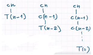
By the Occurrences Tree method we find that:

avg1quicksort

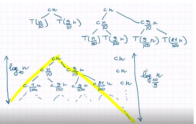
So:

The height of the tree is $h = l o g_{10} (n)$
The longest path from the root, to a leaf here is found by keep going right, $l o g_{10 / 9} (n)$
1. Which is where the recursion stops
The maximum cost of a level is $c n$
1. Every level has cost $c n$ until we reach the depth $l o g_{10} (n)$ where it becomes the upperbound for the cost of a level

Then:

T_{a v e r a g e - c o n s t a n t} (n) \leq c n \cdot l o g_{10 / 9} (n) \Rightarrow T_{a v e r a g e - c o n s t a n t} (n) = O (n l o g (n))

From this we can generalize that:

T (n) = T (α n) + T (n (1 - α)) + c n, where 0 < α < 1 \land c > 0 ⟹ T (n) = Θ (n l o g (n))

Demonstration - Average Case (non-constant)

In the average case where there are two options that keep repeating:

We assume that the input's permutations are i.i.d

T_{a v e r a g e - n o n - c o n s t a n t} (n) = {\begin{matrix} T_{l u c k y} (n) \to L (n) = 2 U (n / 2) + Θ (n) \\ T_{u n l u c k y} (n) \to U (n) = L (n - 1) + Θ (n) \end{matrix}

Then:

L (n) = 2 (L (\frac{n}{2} - 1) + Θ (\frac{n}{2})) + Θ (n) = 2 L (\frac{n}{2} - 1) + 2 Θ (\frac{n}{2})) + Θ (n)

L (n) = 2 L (\frac{n}{2} - 1) + 2 Θ (\frac{n}{2})) + Θ (n) = 2 L (\frac{n}{2} - 1) + Θ (n)

L (n) = 2 L (\frac{n}{2} - 1) + Θ (n) = Θ (n l o g (n))

Avoiding Worst Case: Randomized Version

Instead of choosing $A [r]$ as pivot, we use a random pivot in $A [p \dots r]$

We assume all the keys are distinct

python

#returns random integer between p and r
int randomized_partition(int arr[], int p, int r)
    int i = random(p,r); 
    swap(&arr, i, r); #swap arr[i] and arr[j]
    return partition(arr, p, r);

randomized_quicksort(int arr[], int p, int r)
    if(p < r):
        q = randomized_partition(arr, p, r);
        randomized_quicksort(arr, p, q - 1);
        randomized_quicksort(arr, q + 1, r);

#returns random integer between p and r
int randomized_partition(int arr[], int p, int r)
    int i = random(p,r); 
    swap(&arr, i, r); #swap arr[i] and arr[j]
    return partition(arr, p, r);

randomized_quicksort(int arr[], int p, int r)
    if(p < r):
        q = randomized_partition(arr, p, r);
        randomized_quicksort(arr, p, q - 1);
        randomized_quicksort(arr, q + 1, r);

T_{a v g} (n) = Θ (n l o g (n)) \land T_{w} (n) = Θ (n^{2})

Pros:

$T (n)$ does not depend on the input's order
No assumption on the input's distribution.
No specific input can define the worst case
The random number generator defines the worst case
It is 3 to 4 times faster than the normal version.

Optimization - Insertionsort on small vectors

By using a value m 5 <= m <= 25 to have a range of cases where the insertion sort overrides the main algorithm can help to improve the average case scenario.

Case 1: We can either sort it only if the input is in range

python

quicksort(int * arr, int p, int r)
   if(r - p <= M):
      insertionsort(arr);

quicksort(int * arr, int p, int r)
   if(r - p <= M):
      insertionsort(arr);

Case 2:

python

quicksort(int * arr, int p, int r)
   if(r - p <= M):
      return;

sort(int * arr, int p, int r)
    quicksort(arr, p, r); # partially sorted vectors
    insertionsort(arr); # we sort the rest with insertion sort

quicksort(int * arr, int p, int r)
   if(r - p <= M):
      return;

sort(int * arr, int p, int r)
    quicksort(arr, p, r); # partially sorted vectors
    insertionsort(arr); # we sort the rest with insertion sort

Optimization 2 - Median as pivot

Using a value $m$ the pivot for the quicksort means,

Choosing the median out of three elements inside an unsorted vector:
- A leftmost element
- A rightmost element
- A center element
Swapping it with $A [r]$
Applying the algorithm

Optimization 3 - Dutch Flag (Tri-Partition)

When we find duplicates, not even randomizing the choice of the pivot can help much.

Instead, of dividing the vector in 2 parts we divide it in 3 parts:

Partition with elements $i < x$
Partition with elements $i > x$
Partition with elements $i = x$

This slightly changes the invariant, but the main idea stays the same.

Partition:

Permutation of the elements in $A [p \dots r]$
Returns $q$ and $t$ , $p \leq q \leq t \leq r$
1. $\forall A [i] \in A [q \dots t] ∋^{'} A [i = q] = A [i + 1] = \dots = A [t = i + n]$
2. $\forall A [i] \in A [p \dots q - 1] ∋^{'} A [i] < A [q]$
3. $\forall A [i] \in A [q + 1 \dots r] ∋^{'} A [i] > A [q]$
$T (n) = Θ (r - p)$

python

partition(int * arr, int p, int r)
    int x = arr[r];
    int min = p, eq = p, max = r;

    # Theta(r-p)
    while(eq < max):
        if(arr[eq] < x):
            swap(arr, min, eq);
            eq++;
            min++;
        else if(arr[eq] == x):
            eq++;
        else:
            max--;
            swap(arr, max, eq);

    swap(arr, r, max);
    return [min, max]; #pair

    
quicksort(int * arr, int p, int r)
    if(p < r):
        int[] qt = partition(arr, p, r);
        quicksort(arr, p, q - 1);
        quicksort(arr, t + 1, r);

partition(int * arr, int p, int r)
    int x = arr[r];
    int min = p, eq = p, max = r;

    # Theta(r-p)
    while(eq < max):
        if(arr[eq] < x):
            swap(arr, min, eq);
            eq++;
            min++;
        else if(arr[eq] == x):
            eq++;
        else:
            max--;
            swap(arr, max, eq);

    swap(arr, r, max);
    return [min, max]; #pair

    
quicksort(int * arr, int p, int r)
    if(p < r):
        int[] qt = partition(arr, p, r);
        quicksort(arr, p, q - 1);
        quicksort(arr, t + 1, r);

Invariant

I N V \equiv {\begin{matrix} x = A [r] is always true & \land \\ \forall k \in [p \dots m i n) ∋^{'} A [k] \leq x & \land \\ \forall k \in [m i n \dots e q) ∋^{'} A [k] = x & \land \\ \forall k \in [m a x \dots r) ∋^{'} A [k] > x & \land \\ p \leq m i n \leq e q \leq m a x \leq r & \land \end{matrix}

We obtain something like this:

| < x | = x | ? | > x | x |

|p |min | eq| max | r |

We can confirm this is holds true at all times:

Initialization
Preservation
Conclusion: When the execution ends, we have $e q = m a x$
1. The last two lines swap the pivot $A [r]$ with the first element larger than $x$
2. We obtain the desired partition

I N V [m a x / e q] \equiv {\begin{matrix} x = A [r] is always true & \land \\ \forall k \in [p \dots m i n) ∋^{'} A [k] \leq x & \land \\ \forall k \in [m i n \dots m a x) ∋^{'} A [k] = x & \land \\ \forall k \in [m a x \dots r) ∋^{'} A [k] > x & \land \\ p \leq m i n \leq m a x \leq r & \land \end{matrix}

The result is:

| < x | = x | > x | x |

|p |min | max | r |

Complexity

If all the elements are equal

T (n) = Θ (n = r - p + 1)

Conclusion

Pro:

In-Loco
Worst Case is very rare, and normally it is very efficient
Randomizing the pivot is a solution for when input is sorted
Tri-partition improves the computing complexity

Con:

Worst Case T(n) = O(n**2)
Not Stable
Not adaptive: slow when input is already sorted (asc/desc) or all the elements have equal values

Extra Credits

[1] CSE Stack - Quick Sort

Quick Sort ​

Idea ​

The Algorithm - Divide et Impera ​

Invariant ​

Time Complexity ​

Demonstration - Worst Case ​

Demonstration - Best Case ​

Demonstration - Average Case (constant) ​

Demonstration - Average Case (non-constant) ​

Avoiding Worst Case: Randomized Version ​

Optimization - Insertionsort on small vectors ​

Optimization 2 - Median as pivot ​

Optimization 3 - Dutch Flag (Tri-Partition) ​

Invariant ​

Complexity ​

Conclusion ​

Extra Credits ​

Quick Sort

Idea

The Algorithm - Divide et Impera

Invariant

Time Complexity

Demonstration - Worst Case

Demonstration - Best Case

Demonstration - Average Case (constant)

Demonstration - Average Case (non-constant)

Avoiding Worst Case: Randomized Version

Optimization - Insertionsort on small vectors

Optimization 2 - Median as pivot

Optimization 3 - Dutch Flag (Tri-Partition)

Invariant

Complexity

Conclusion

Extra Credits